


Kirchhoff's Laws: Complete Guide with Circuit Analysis Examples & Calculations
- Admin: IDAR Mohamed
- 22 Oct 2024
- 0
Kirchhoff's Laws are fundamental principles in electrical engineering that every student and professional must master for effective circuit analysis. These two simple yet powerful laws - Kirchhoff's Current Law (KCL) and Kirchhoff's Voltage Law (KVL) - provide the foundation for solving complex electrical networks and are essential for understanding how current flows and voltage distributes in electrical circuits.
Whether you're designing power distribution systems, analyzing electronic circuit designs, or working with AC circuit analysis, Kirchhoff's Laws are your go-to tools for accurate calculations and reliable results.
Understanding Kirchhoff's Laws: The Foundation of Circuit Analysis
Kirchhoff's Laws consist of two fundamental principles that govern electrical circuits:
1. Kirchhoff's Current Law (KCL) - Node Analysis
Statement: The algebraic sum of all currents entering and leaving any node (junction) in a circuit equals zero.
Mathematical Expression:
Or alternatively:
Physical Basis: Based on the conservation of electric charge - charge cannot accumulate at any point in a circuit.
2. Kirchhoff's Voltage Law (KVL) - Loop Analysis
Statement: The algebraic sum of all voltage drops and rises around any closed loop in a circuit equals zero.
Mathematical Expression:
Physical Basis: Based on the conservation of energy - the energy gained by a charge moving around a closed loop must equal the energy lost.
Step-by-Step Circuit Analysis Using Kirchhoff's Laws
Example 1: Simple Series-Parallel Circuit Analysis
Let's solve a practical circuit with the following components:
- Voltage source: V = 12V
- Resistor R₁ = 4Ω (series)
- Resistor R₂ = 6Ω (parallel branch)
- Resistor R₃ = 3Ω (parallel branch)
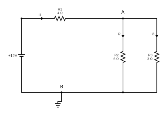
Step 1: Identify Nodes and Loops
- Node A: Junction where R₁ connects to parallel branches
- Node B: Common ground point
- Loop 1: V - R₁ - R₂ (through R₂ branch)
- Loop 2: R₂ - R₃ (between parallel branches)
Step 2: Apply KCL at Node A
Let's define:
- I₁ = current through R₁
- I₂ = current through R₂
- I₃ = current through R₃
Applying KCL at Node A:
Step 3: Apply KVL in Loop 1
Going clockwise around Loop 1:
Step 4: Apply KVL in Loop 2
Around the parallel branch loop:
Step 5: Solve the System of Equations
Substituting Equation 2 into the KCL equation:
Substituting into Equation 1:
Therefore:
- I₂ = 0.667A
- I₃ = 2 × 0.667 = 1.333A
- I₁ = 3 × 0.667 = 2A
Step 6: Verify Using Power Balance
Total power supplied: P = VI₁ = 12V × 2A = 24W
Power dissipated:
- P₁ = I₁²R₁ = (2)² × 4 = 16W
- P₂ = I₂²R₂ = (0.667)² × 6 = 2.67W
- P₃ = I₃²R₃ = (1.333)² × 3 = 5.33W
- Total = 16 + 2.67 + 5.33 = 24W ✓
Example 2: Complex Multi-Loop Circuit
Mesh Analysis Using Kirchhoff's Voltage Law (KVL)
Mesh analysis is a systematic method for solving electrical circuits using Kirchhoff's Voltage Law (KVL). This technique is particularly useful for circuits with multiple loops and current sources.
Circuit Analysis Example
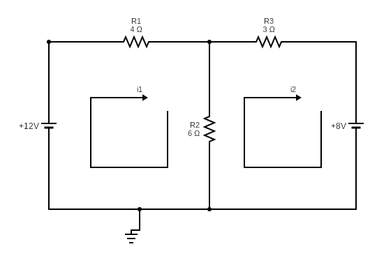
Let's analyze a two-mesh circuit with multiple voltage sources and resistors to demonstrate the complete mesh analysis process.
Given Circuit Parameters:
- V₁ = 12V (voltage source)
- V₂ = 8V (voltage source)
- R₁ = 4Ω (resistor)
- R₂ = 6Ω (resistor)
- R₃ = 3Ω (resistor)
Step 1: Identify Meshes and Assign Mesh Currents
We have two meshes in this circuit:
- Mesh 1 (i₁): Left loop containing V₁, R₁, and R₂
- Mesh 2 (i₂): Right loop containing R₂, V₂, and R₃
Both mesh currents are assumed to flow clockwise.
info
When assigning mesh currents, it's important to be consistent with the direction (all clockwise or all counterclockwise) to avoid sign errors in your equations.
Step 2: Apply KVL to Mesh 1
Starting from the top and going clockwise:
- Voltage rises: +V₁ = +12V
- Voltage drops: -i₁R₁ - (i₁ - i₂)R₂
Applying KVL:
Substituting the given values:
Expanding:
Simplifying:
Step 3: Apply KVL to Mesh 2
Starting from the top and going clockwise:
- Voltage rises: +V₂ = +8V
- Voltage drops: -(i₂ - i₁)R₂ - i₂R₃
Applying KVL:
Substituting the given values:
Expanding:
Simplifying:
Step 4: Solve the System of Equations
We now have two equations with two unknowns:
Rearranging:
- From equation (1):
- From equation (2):
Multiply equation (2) by 2:
Subtract equation (1) from equation (3):
Substitute into equation (1):
Step 5: Calculate Individual Branch Currents
Now we can determine the current through each component:
| Component | Current | Voltage Drop |
|---|---|---|
| R₁ | A | V |
| R₂ | A | V |
| R₃ | A | V |
Solution Verification
Let's verify our solution by checking both KVL equations:
Mesh 1 verification:
Mesh 2 verification:
Both equations are satisfied, confirming our solution is correct!
Final Results
- Mesh Current 1 (i₁): 2 A (clockwise)
- Mesh Current 2 (i₂): 4/3 A ≈ 1.33 A (clockwise)
- Current through R₁: 2 A (left to right)
- Current through R₂: 2/3 A ≈ 0.67 A (top to bottom)
- Current through R₃: 4/3 A ≈ 1.33 A (right to left)
Key Points to Remember
- Consistent Direction: Always define mesh currents consistently (all clockwise or all counterclockwise)
- Shared Components: For shared resistors, the current is the algebraic sum of mesh currents
- Voltage Sources: Add positive voltage when traversed from + to - terminal
- Resistor Drops: Always have voltage drops in the direction of current flow
- Verification: Always verify your solution by substituting back into the original equations
Applications and Benefits
Mesh analysis is particularly effective for:
- Circuits with multiple voltage sources
- Planar circuits (can be drawn without crossing wires)
- When you need to find mesh currents directly
- Academic and theoretical circuit analysis
info
While mesh analysis is powerful, for circuits with many current sources, nodal analysis might be more efficient. Choose the method that results in fewer equations to solve.
Advanced Applications of Kirchhoff's Laws
1. AC Circuit Analysis
When working with alternating current circuits, Kirchhoff's Laws apply to:
- Instantaneous values: KCL and KVL hold at every instant
- Phasor analysis: Using complex numbers for sinusoidal steady-state
- RMS values: For power calculations in AC systems
2. Nodal Voltage Method
This systematic approach uses KCL primarily:
Steps for Nodal Analysis:
- Select reference node (ground)
- Identify node voltages
- Apply KCL at each non-reference node
- Express currents using Ohm's law
- Solve resulting equations
3. Mesh Current Method
This approach uses KVL primarily:
Steps for Mesh Analysis:
- Identify all meshes (loops)
- Assign mesh currents
- Apply KVL around each mesh
- Express voltages using Ohm's law
- Solve for mesh currents
Practical Applications in Electrical Engineering
Power Distribution Systems
In electrical power systems, Kirchhoff's Laws ensure:
- Load balancing across distribution networks
- Fault analysis in transmission lines
- Power flow calculations in electrical grids
Electronic Circuit Design
For electronic components and circuit design:
- Amplifier analysis using operational amplifiers
- Filter circuit design for signal processing
- Digital logic circuits and microcontroller interfacing
Circuit Simulation and Analysis
Modern circuit simulation software like SPICE uses Kirchhoff's Laws as the foundation for:
- SPICE modeling of electronic circuits
- Transient analysis for time-domain behavior
- Frequency response analysis
Troubleshooting Common Circuit Problems
Problem-Solving Strategy
- Identify the circuit topology (series, parallel, or combination)
- Choose analysis method (nodal or mesh analysis)
- Apply appropriate Kirchhoff's Law
- Set up equations systematically
- Solve and verify results
Circuit Analysis Comparison Table
| Method | Primary Law Used | Best For | Variables Solved |
|---|---|---|---|
| Nodal Analysis | KCL (Current Law) | Circuits with fewer nodes | Node voltages |
| Mesh Analysis | KVL (Voltage Law) | Circuits with fewer loops | Loop currents |
| Branch Analysis | Both KCL & KVL | Simple circuits | Branch currents/voltages |
| Superposition | Both (applied separately) | Multi-source circuits | Individual source effects |
Advanced Circuit Analysis Techniques
Thévenin and Norton Equivalent Circuits
Using Kirchhoff's Laws with Thévenin's theorem:
- Simplify complex networks
- Analyze load variations
- Design matching networks
Superposition Principle
When dealing with multi-source circuits:
- Apply Kirchhoff's Laws to each source individually
- Sum the individual responses
- Verify using complete circuit analysis
Real-World Circuit Examples
Example 3: LED Circuit Analysis
For LED circuit design:
- Forward voltage drop: V_LED = 2.2V
- Supply voltage: V_s = 9V
- Desired current: I_LED = 20mA
- Required resistance: R = (9V - 2.2V) / 0.02A = 340Ω
Example 4: Battery Charging Circuit
In battery management systems:
- Apply KVL to determine charging current
- Use KCL for current distribution in parallel battery banks
- Calculate power dissipation in charging resistors
Circuit Analysis Software and Tools
Modern electrical engineers use various tools that implement Kirchhoff's Laws:
- LTSpice - Free SPICE simulator
- Multisim - Educational circuit simulation
- PSpice - Professional circuit analysis
- MATLAB Simulink - System-level modeling
- KiCad - Open-source PCB design with simulation
These tools automate the application of Kirchhoff's Laws for complex circuits with hundreds or thousands of components.
Best Practices for Circuit Analysis
1. Systematic Approach
- Always define current directions and voltage polarities clearly
- Use consistent sign conventions throughout the analysis
- Label all nodes and components systematically
2. Verification Methods
- Check that KCL is satisfied at each node
- Verify that KVL equals zero around each loop
- Confirm power balance (power supplied = power consumed)
3. Common Pitfalls to Avoid
- Mixing up current directions in KCL equations
- Incorrect voltage polarity in KVL loops
- Forgetting to include all circuit elements
- Using dependent variables without establishing relationships
Conclusion: Mastering Circuit Analysis with Kirchhoff's Laws
Kirchhoff's Current and Voltage Laws remain the cornerstone of electrical circuit analysis, providing the theoretical foundation for understanding everything from simple resistor circuits to complex power electronic systems. Whether you're working on Arduino projects, designing PCB layouts, or analyzing industrial electrical systems, these fundamental laws will guide your analysis and ensure accurate results.
The key to mastering circuit analysis lies in consistent practice with increasingly complex circuits, understanding when to apply each law, and developing the ability to set up and solve systems of equations efficiently. With the step-by-step examples and practical applications covered in this guide, you now have the tools to tackle any circuit analysis challenge with confidence.
Ready to advance your electrical engineering skills? Explore our comprehensive guides on advanced circuit analysis and electrical engineering fundamentals to deepen your understanding of these essential concepts.
🔗 Related Posts
- Electric Current: A Comprehensive Guide
- Electrical Resistance and How to Calculate It
- Mastering PCB Design and Techniques Wire size Calculator - complete guide
Helpful Calculators
- Resistor Color Code Calculator
- Series Parallel Resistance Calculator
- Ohm's Law Calculator
- Voltage Drop Calculator
Credits
- Photo by Chris Ried on Unsplash
⭐ Was this article helpful?
IDAR Mohamed
Electrical Engineer
Electrical Engineer specialized in power systems, electrical installations, and energy efficiency. Passionate about simplifying complex electrical concepts into practical guides. (University of applied sciences graduate, with experience in HV/LV systems and industrial installations.)
- Kirchhoff's Laws
- Circuit Analysis
- Electrical Engineering
- KCL KVL
- Node Voltage Method
- Mesh Current Method
- Circuit Calculations
- Electrical Circuits