Load Flow Analysis: Complete Guide to Power Flow Calculations with Newton-Raphson & Gauss-Seidel Methods

Load flow analysis, also known as power flow analysis, is the cornerstone of power system planning, operation, and optimization. This computational technique determines the steady-state operating conditions of an electrical power network by calculating voltage magnitudes, phase angles, active power, and reactive power at each bus in the system. Whether you're designing a new substation, planning system expansions, or optimizing power generation dispatch, load flow analysis provides the essential data needed for informed decision-making.

Understanding load flow analysis is critical for electrical engineers working in power utilities, renewable energy integration, industrial power systems, and smart grid applications. This comprehensive guide will walk you through the fundamental concepts, solution methods, practical calculations, and real-world applications of load flow analysis in modern power systems.

Table of Contents

1. Understanding Load Flow Analysis Fundamentals
2. Bus Classification in Power Systems
3. Y-Bus Admittance Matrix Formation
4. Load Flow Solution Methods
5. Newton-Raphson Method: Step-by-Step Guide
6. Gauss-Seidel Method Explained
7. Practical Load Flow Calculations
8. Software Tools for Load Flow Analysis
9. Applications and Case Studies

Understanding Load Flow Analysis Fundamentals

What is Load Flow Analysis?

Load flow analysis is a numerical method used to calculate the steady-state electrical quantities in a power system network. It determines how power flows through transmission lines, transformers, and other components while maintaining voltage levels within acceptable limits.

Key Objectives of Load Flow Analysis:

• Calculate bus voltage magnitudes and phase angles
• Determine active and reactive power flows in transmission lines
• Identify system losses and efficiency
• Evaluate voltage profiles across the network
• Assess system loading and identify overloaded equipment
• Verify system stability margins

Why Load Flow Analysis Matters

Power system engineers rely on load flow studies for numerous critical applications:

System Planning and Design:

• Sizing transmission lines and transformers
• Planning new generation and load connections
• Evaluating system expansion scenarios
• Optimizing network topology

Operational Analysis:

• Real-time system monitoring and control
• Economic dispatch optimization
• Contingency analysis (N-1, N-2 security)
• Voltage and reactive power control

Reliability Studies:

• Identifying weak points in the network
• Assessing voltage stability margins
• Evaluating system response to disturbances
• Planning maintenance outages

Power Flow Equations

The foundation of load flow analysis rests on the power balance equations at each bus in the network.

Complex Power at Bus i:

$$S_i = P_i + jQ_i = V_i \sum_{k=1}^{n} Y_{ik}^* V_k^*$$

Where:

• $S_i$ = Complex power at bus i
• $P_i$ = Active power (watts)
• $Q_i$ = Reactive power (vars)
• $V_i$ = Voltage at bus i
• $Y_{ik}$ = Element of Y-bus admittance matrix
• $n$ = Total number of buses

Expanded Power Equations:

Active Power:

$$P_i = \sum_{k=1}^{n} |V_i||V_k||Y_{ik}| \cos(\theta_{ik} - \delta_i + \delta_k)$$

Reactive Power:

$$Q_i = \sum_{k=1}^{n} |V_i||V_k||Y_{ik}| \sin(\theta_{ik} - \delta_i + \delta_k)$$

Where:

• $\theta_{ik}$ = Angle of admittance element $Y_{ik}$
• $\delta_i, \delta_k$ = Voltage angles at buses i and k

These nonlinear equations form the basis for all load flow solution methods.

Bus Classification in Power Systems

Understanding bus types is fundamental to setting up and solving load flow problems. Each bus in the system is classified based on which quantities are specified and which need to be calculated.

The Three Bus Types

1. Slack Bus (Swing Bus or Reference Bus)

Characteristics:

• Specified: Voltage magnitude ($|V|$) and angle ($\delta$)
• Calculated: Active power ($P$) and reactive power ($Q$)
• Symbol: Usually Bus 1
• Purpose: Provides system balance and reference angle

Physical Significance: The slack bus represents the generator that accommodates the mismatch between total generation and total load plus losses. Since system losses are unknown before solving the load flow, one bus must be designated to supply or absorb this difference.

Typical Specification:

• Voltage magnitude: 1.0 per unit (p.u.)
• Voltage angle: 0° (reference)

2. PV Bus (Generator Bus or Voltage-Controlled Bus)

Characteristics:

• Specified: Active power ($P$) and voltage magnitude ($|V|$)
• Calculated: Reactive power ($Q$) and voltage angle ($\delta$)
• Symbol: Usually Bus 2, 3, etc.
• Purpose: Represents generators with voltage control

Physical Significance: PV buses represent synchronous generators or synchronous condensers that can maintain constant voltage through automatic voltage regulators (AVRs) while supplying specified active power.

Typical Specification:

• Active power: Based on generation schedule
• Voltage magnitude: 1.0-1.05 p.u. (maintained by AVR)

Operating Limits: Generators have reactive power limits:

• $Q_{min} \leq Q \leq Q_{max}$

If calculated $Q$ exceeds limits during iterations, the bus may be converted to a PQ bus with $Q$ fixed at the limit.

3. PQ Bus (Load Bus)

Characteristics:

• Specified: Active power ($P$) and reactive power ($Q$)
• Calculated: Voltage magnitude ($|V|$) and angle ($\delta$)
• Symbol: Most buses in the system
• Purpose: Represents loads and uncontrolled generation

Physical Significance: PQ buses represent constant power loads, which is a reasonable approximation for most industrial and commercial loads. They can also represent small generators without voltage control.

Typical Specification:

• Active power: Load demand (negative)
• Reactive power: Load demand (negative)

Bus Classification Summary Table

Bus Type	Known Variables	Unknown Variables	Quantity
Slack	$\|V\|, \delta$	$P, Q$	1 per system
PV	$P, \|V\|$	$Q, \delta$	Number of generators - 1
PQ	$P, Q$	$\|V\|, \delta$	All load buses

Example Bus Classification

Consider a 4-bus system with the following specifications:

Bus	Type	P (MW)	Q (MVAr)	|V| (p.u.)	δ (degrees)
1	Slack	?	?	1.05	0.0
2	PV	50	?	1.04	?
3	PQ	-80	-40	?	?
4	PQ	-60	-30	?	?

This system has:

• 1 slack bus (provides reference)
• 1 PV bus (generator with voltage control)
• 2 PQ buses (load buses)

Y-Bus Admittance Matrix Formation

The Y-bus (admittance matrix) is a fundamental component in load flow analysis, representing the electrical network in matrix form.

What is the Y-Bus Matrix?

The Y-bus is a sparse, complex matrix that relates bus currents to bus voltages:

$$[I] = [Y_{bus}][V]$$

Where:

• $[I]$ = Bus current injection vector
• $[Y_{bus}]$ = System admittance matrix
• $[V]$ = Bus voltage vector

Y-Bus Matrix Structure

For an n-bus system:

$$Y_{bus} = \begin{bmatrix} Y_{11} & Y_{12} & \cdots & Y_{1n} \\ Y_{21} & Y_{22} & \cdots & Y_{2n} \\ \vdots & \vdots & \ddots & \vdots \\ Y_{n1} & Y_{n2} & \cdots & Y_{nn} \end{bmatrix}$$

Diagonal Elements (Self-admittance):

$$Y_{ii} = \sum_{k=1, k \neq i}^{n} y_{ik} + y_{i0}$$

Where:

• $y_{ik}$ = Series admittance of line connecting buses i and k
• $y_{i0}$ = Shunt admittance at bus i

Off-Diagonal Elements (Mutual admittance):

$$Y_{ik} = -y_{ik}$$

Where $y_{ik}$ is the series admittance between buses i and k.

Y-Bus Formation Example

Consider a simple 3-bus system:

3-Bus Power System: Line 1–2 (0.02 + j0.04 p.u.), Line 2–3 (0.0125 + j0.025 p.u.), Line 1–3 (0.01 + j0.03 p.u.), with shunt capacitance y₂₀ = j0.05 p.u.

System Data:

• Line 1-2: $z_{12} = 0.02 + j0.04$ p.u.
• Line 2-3: $z_{23} = 0.0125 + j0.025$ p.u.
• Line 1-3: $z_{13} = 0.01 + j0.03$ p.u.
• Shunt capacitance at bus 2: $y_{20} = j0.05$ p.u.

Step 1: Calculate Series Admittances

$$y_{12} = \frac{1}{z_{12}} = \frac{1}{0.02 + j0.04} = 10 - j20 \text{ p.u.}$$ $$y_{23} = \frac{1}{z_{23}} = \frac{1}{0.0125 + j0.025} = 16 - j32 \text{ p.u.}$$ $$y_{13} = \frac{1}{z_{13}} = \frac{1}{0.01 + j0.03} = 10 - j30 \text{ p.u.}$$

Step 2: Calculate Diagonal Elements

$$Y_{11} = y_{12} + y_{13} = (10 - j20) + (10 - j30) = 20 - j50 \text{ p.u.}$$ $$Y_{22} = y_{12} + y_{23} + y_{20} = (10 - j20) + (16 - j32) + j0.05 = 26 - j51.95 \text{ p.u.}$$ $$Y_{33} = y_{13} + y_{23} = (10 - j30) + (16 - j32) = 26 - j62 \text{ p.u.}$$

Step 3: Calculate Off-Diagonal Elements

$$Y_{12} = Y_{21} = -y_{12} = -10 + j20 \text{ p.u.}$$ $$Y_{23} = Y_{32} = -y_{23} = -16 + j32 \text{ p.u.}$$ $$Y_{13} = Y_{31} = -y_{13} = -10 + j30 \text{ p.u.}$$

Complete Y-Bus Matrix:

$$Y_{bus} = \begin{bmatrix} 20-j50 & -10+j20 & -10+j30 \\ -10+j20 & 26-j51.95 & -16+j32 \\ -10+j30 & -16+j32 & 26-j62 \end{bmatrix}$$

Y-Bus Properties

Key Characteristics:

1. Symmetry: $Y_{ik} = Y_{ki}$ for passive networks
2. Sparsity: Most elements are zero (no direct connection)
3. Diagonal dominance: $|Y_{ii}| > \sum_{k \neq i} |Y_{ik}|$
4. Complex values: Real part = conductance, imaginary part = susceptance

Load Flow Solution Methods

Load flow problems are solved using iterative numerical methods due to the nonlinear nature of the power flow equations. Three main methods are commonly used in practice.

Comparison of Solution Methods

Method	Convergence Speed	Memory Requirements	Reliability	Best Application
Gauss-Seidel	Slow (10-50 iterations)	Low	Good for small systems	Educational purposes
Newton-Raphson	Fast (3-5 iterations)	High	Excellent	Large systems (most common)
Fast Decoupled	Very fast (3-4 iterations)	Moderate	Good for well-conditioned	Contingency analysis

Method Selection Criteria

Choose Gauss-Seidel when:

• System size is small (< 10 buses)
• Memory is limited
• Simple implementation is needed
• Educational/learning purposes

Choose Newton-Raphson when:

• System size is large (> 10 buses)
• Fast convergence is critical
• High accuracy is required
• Most practical applications

Choose Fast Decoupled when:

• Multiple load flow solutions needed (contingency studies)
• System is well-conditioned (high X/R ratio)
• Speed is paramount
• Real-time applications

Newton-Raphson Method: Step-by-Step Guide

The Newton-Raphson method is the most widely used technique for load flow analysis due to its quadratic convergence characteristics and reliability.

Newton-Raphson Algorithm Overview

The method linearizes the nonlinear power flow equations using Taylor series expansion and solves iteratively:

$$\begin{bmatrix} \Delta P \\ \Delta Q \end{bmatrix} = \begin{bmatrix} J_1 & J_2 \\ J_3 & J_4 \end{bmatrix} \begin{bmatrix} \Delta \delta \\ \Delta |V| \end{bmatrix}$$

Where:

• $\Delta P, \Delta Q$ = Power mismatches
• $\Delta \delta, \Delta |V|$ = Corrections to voltage angles and magnitudes
• $J_1, J_2, J_3, J_4$ = Jacobian matrix sub-matrices

The Jacobian Matrix

The Jacobian contains partial derivatives of power equations with respect to voltage variables:

J1 Matrix ($∂P/∂δ$):

$$J_{1(i,k)} = \frac{\partial P_i}{\partial \delta_k} = |V_i||V_k||Y_{ik}| \sin(\theta_{ik} - \delta_i + \delta_k)$$

For diagonal elements (i = k):

$$J_{1(i,i)} = -Q_i - |V_i|^2 B_{ii}$$

J2 Matrix ($∂P/∂|V|$):

$$J_{2(i,k)} = \frac{\partial P_i}{\partial |V_k|} = |V_i||Y_{ik}| \cos(\theta_{ik} - \delta_i + \delta_k)$$

For diagonal elements:

$$J_{2(i,i)} = P_i/|V_i| + |V_i| G_{ii}$$

J3 Matrix ($∂Q/∂δ$):

$$J_{3(i,k)} = \frac{\partial Q_i}{\partial \delta_k} = -|V_i||V_k||Y_{ik}| \cos(\theta_{ik} - \delta_i + \delta_k)$$

For diagonal elements:

$$J_{3(i,i)} = P_i - |V_i|^2 G_{ii}$$

J4 Matrix ($∂Q/∂|V|$):

$$J_{4(i,k)} = \frac{\partial Q_i}{\partial |V_k|} = |V_i||Y_{ik}| \sin(\theta_{ik} - \delta_i + \delta_k)$$

For diagonal elements:

$$J_{4(i,i)} = Q_i/|V_i| - |V_i| B_{ii}$$

Newton-Raphson Algorithm Steps

Step 1: Initialize

• Set all PQ bus voltages to 1.0 ∠ 0° p.u.
• Set all PV bus angles to 0°
• Set iteration counter k = 0

Step 2: Calculate Power Mismatches

For each bus i (except slack):

$$\Delta P_i^{(k)} = P_i^{spec} - P_i^{(k)}$$

For each PQ bus:

$$\Delta Q_i^{(k)} = Q_i^{spec} - Q_i^{(k)}$$

Step 3: Check Convergence

If $|\Delta P_i^{(k)}| < \epsilon$ and $|\Delta Q_i^{(k)}| < \epsilon$ for all buses:

• Solution converged → STOP
• Else → Continue

Typical tolerance: $\epsilon = 0.001$ p.u.

Step 4: Form Jacobian Matrix

Calculate all elements of J1, J2, J3, J4 using current voltage estimates.

Step 5: Solve Linear System

$$\begin{bmatrix} \Delta \delta^{(k)} \\ \Delta |V|^{(k)} \end{bmatrix} = \begin{bmatrix} J \end{bmatrix}^{-1} \begin{bmatrix} \Delta P^{(k)} \\ \Delta Q^{(k)} \end{bmatrix}$$

Step 6: Update Voltages

For PV and PQ buses:

$$\delta_i^{(k+1)} = \delta_i^{(k)} + \Delta \delta_i^{(k)}$$

For PQ buses:

$$|V_i|^{(k+1)} = |V_i|^{(k)} + \Delta |V_i|^{(k)}$$

Step 7: Increment and Repeat

• Set k = k + 1
• Return to Step 2

Newton-Raphson Example Problem

Let's solve a 3-bus system load flow problem:

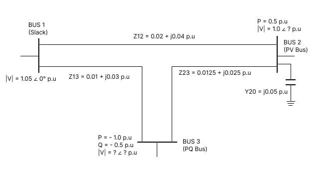
Newton–Raphson Load Flow Example for a 3-Bus Power System — Bus 1 (Slack), Bus 2 (PV, P = 0.5 p.u.), Bus 3 (PQ, P = −1.0 p.u., Q = −0.5 p.u.) with corresponding voltage magnitudes and phase angles.

System Data:

Bus	Type	P (p.u.)	Q (p.u.)	|V| (p.u.)	δ
1	Slack	-	-	1.05	0°
2	PV	0.5	-	1.00	?
3	PQ	-1.0	-0.5	?	?

Y-Bus Matrix (from previous example):

$$Y_{bus} = \begin{bmatrix} 20-j50 & -10+j20 & -10+j30 \\ -10+j20 & 26-j51.95 & -16+j32 \\ -10+j30 & -16+j32 & 26-j62 \end{bmatrix}$$

Iteration 1: Initialize

• $V_2 = 1.00 \angle 0°$ p.u.
• $V_3 = 1.00 \angle 0°$ p.u.

Calculate Power at Bus 2:

$$P_2^{calc} = |V_2| \sum_{k=1}^{3} |V_k||Y_{2k}| \cos(\theta_{2k} - \delta_2 + \delta_k)$$

After calculation: $P_2^{calc} = 0.526$ p.u.

Calculate Power Mismatch:

$$\Delta P_2 = P_2^{spec} - P_2^{calc} = 0.5 - 0.526 = -0.026 \text{ p.u.}$$

Similarly for bus 3:

$$\Delta P_3 = -1.0 - P_3^{calc}$$ $$\Delta Q_3 = -0.5 - Q_3^{calc}$$

Form Jacobian and Solve: The process continues iteratively until convergence (typically 3-5 iterations).

Final Solution (after convergence):

• Bus 2: $\delta_2 = -2.5°$, $Q_2 = 0.32$ p.u.
• Bus 3: $|V_3| = 0.98$ p.u., $\delta_3 = -4.2°$

Gauss-Seidel Method Explained

The Gauss-Seidel method is an iterative technique that solves load flow problems by updating bus voltages sequentially.

Gauss-Seidel Algorithm

Voltage Update Formula:

For PQ buses:

$$V_i^{(k+1)} = \frac{1}{Y_{ii}} \left[ \frac{P_i - jQ_i}{V_i^{(k)*}} - \sum_{j=1, j \neq i}^{n} Y_{ij} V_j^{(k+1)} \right]$$

For PV buses:

$$V_i^{(k+1)} = \frac{1}{Y_{ii}} \left[ \frac{P_i - jQ_i^{(k)}}{V_i^{(k)*}} - \sum_{j=1, j \neq i}^{n} Y_{ij} V_j^{(k+1)} \right]$$

Then adjust magnitude:

$$V_i^{(k+1)} = |V_i^{spec}| \angle \arg(V_i^{(k+1)})$$

Acceleration Factor

To improve convergence, an acceleration factor α is often used:

$$V_i^{(k+1)} = V_i^{(k)} + \alpha(V_i^{new} - V_i^{(k)})$$

Typical values: $1.3 \leq \alpha \leq 1.6$

Gauss-Seidel vs Newton-Raphson

Advantages of Gauss-Seidel:

• Simple implementation
• Low memory requirements
• Good for small systems
• No matrix inversion needed

Disadvantages:

• Slow convergence (linear)
• May not converge for ill-conditioned systems
• More iterations required

Practical Load Flow Calculations

Load Flow Analysis Workflow

1. Data Collection:

• Network topology (line connections)
• Line impedances and shunt admittances
• Transformer tap settings and impedances
• Generator specifications (P, V limits)
• Load data (P, Q at each bus)
• Base MVA for per-unit system

2. System Modeling:

• Convert all data to per-unit values
• Form Y-bus admittance matrix
• Classify buses (slack, PV, PQ)
• Set initial voltage estimates

3. Load Flow Solution:

• Choose solution method (Newton-Raphson recommended)
• Run iterative solution
• Check for convergence
• Handle generator reactive power limits

4. Results Analysis:

• Calculate line flows and losses
• Check voltage profile compliance
• Identify overloaded equipment
• Verify generator limits
• Calculate total system losses

Handling Generator Limits

During iterations, check PV bus reactive power:

$$Q_{min} \leq Q_{calc} \leq Q_{max}$$

If violated:

1. Convert PV bus to PQ bus
2. Set Q to violated limit
3. Continue iterations
4. Voltage will now vary

Voltage Regulation Considerations

Acceptable Voltage Ranges:

• Transmission systems: ±5% (0.95-1.05 p.u.)
• Distribution systems: ±10% (0.90-1.10 p.u.)
• Critical loads: ±3% (0.97-1.03 p.u.)

Voltage Control Methods:

• Generator excitation control
• Transformer tap changing
• Capacitor bank switching
• Static VAR compensators (SVC)
• STATCOM devices

Software Selection Guide

Application	Recommended Software	Key Feature
Education	PowerWorld, MATPOWER	Learning focus
Utility Planning	PSS/E, PowerFactory	Large system handling
Industrial	ETAP, SKM PowerTools	Equipment library
Distribution	OpenDSS, Cymdist	Distribution modeling
Research	MATPOWER, PowerFactory	Flexibility

Applications and Case Studies

Case Study 1: Distribution System Planning

Scenario: A utility needs to evaluate adding a new industrial load of 5 MW, 3 MVAr to an existing distribution system.

Load Flow Analysis Steps:

1. Model Existing System:

   • 10 buses, 12 distribution lines
   • Base case with existing loads

2. Add New Load:

   • Connect to nearest appropriate bus
   • Model new connection impedance

3. Run Load Flow:

   • Check voltage profile
   • Identify overloaded feeders
   • Calculate additional losses

Results:

• Voltage at new load bus: 0.93 p.u. (acceptable)
• Existing feeder loading increased to 92%
• Additional system losses: 45 kW
• Recommendation: Proceed with connection, monitor feeder loading

Case Study 2: Renewable Energy Integration

Scenario: Connecting a 50 MW solar farm to the transmission grid.

Analysis Requirements:

• Steady-state voltage impact
• Reverse power flow capability
• Voltage regulation needs
• Reactive power requirements

Load Flow Findings:

• Solar generation causes voltage rise (1.04 p.u.)
• Need for dynamic voltage support (STATCOM)
• Transmission line utilization changes
• Reactive power absorption required during high generation

Case Study 3: Transmission System Expansion

Scenario: Planning a new 230 kV transmission line to relieve congestion.

Load Flow Studies:

• Base case load flow (existing system)
• Future load growth scenarios (5, 10, 15 years)
• Contingency analysis (N-1 criterion)
• Alternative routing options

Optimization Objectives:

• Minimize transmission losses
• Maintain voltage within limits
• Ensure thermal limits not exceeded
• Cost-effective solution

Results:

• Optimal line routing identified
• Voltage profile improved by 3%
• System losses reduced by 2.5 MW
• N-1 security criteria met

Real-World Application: Daily Operations

Utility Control Center Usage:

• Every 5-15 minutes: State estimator runs load flow
• Continuously: Monitor voltage violations
• Hourly: Economic dispatch optimization
• Pre-outage: Contingency analysis using load flow
• Post-disturbance: Verify system stability

Advanced Load Flow Topics

Fast Decoupled Load Flow (FDLF)

The FDLF method exploits the weak coupling between P-δ and Q-|V| in power systems to simplify the Newton-Raphson Jacobian.

Key Assumptions:

1. $\cos(\delta_i - \delta_k) \approx 1$ (small angle differences)
2. $\sin(\delta_i - \delta_k) \approx 0$
3. $Q_i \ll |V_i|^2 B_{ii}$ (reactive power mainly depends on susceptance)
4. $G_{ik} \ll B_{ik}$ (high X/R ratio)

Decoupled Equations:

$$[\Delta P] = [B'][\Delta \delta]$$ $$[\Delta Q] = [B''][\Delta |V|]$$

Where $[B']$ and $[B'']$ are constant imaginary parts of the Jacobian.

Advantages:

• Constant matrices (calculated once)
• Separate P-δ and Q-V solutions
• 2-3 times faster than Newton-Raphson per iteration
• Excellent for contingency studies

When to Use FDLF:

• Well-conditioned transmission systems
• High X/R ratios (typical for HV systems)
• Multiple load flow solutions needed
• Real-time applications

Three-Phase Load Flow

For unbalanced distribution systems, three-phase load flow is required:

Characteristics:

• Models each phase separately
• Accounts for unbalanced loads
• Considers neutral conductor
• Phase-to-phase coupling

Applications:

• Distribution system analysis
• Unbalanced fault studies
• Phase balancing studies
• DG integration in distribution

Voltage Stability Analysis

Load flow analysis is essential for voltage stability assessment:

PV Curves (Nose Curves):

• Plot voltage vs. increasing load
• Identify maximum loadability point
• Determine stability margins

Voltage Stability Indicators:

• Minimum singular value of Jacobian
• Voltage sensitivity factors
• L-index (loading index)

Critical Loading:

$$P_{critical} = P_{base} \times \text{Loading Factor}$$

When system approaches voltage collapse, load flow may not converge.

Load Flow Analysis Best Practices

Model Accuracy Requirements

Transmission System Modeling:

• Include all lines and transformers
• Model shunt reactors and capacitors
• Accurate generator data including limits
• Proper representation of FACTS devices

Distribution System Modeling:

• Include service transformers
• Model voltage regulators and LTCs
• Represent distributed generation
• Account for unbalanced loads

Convergence Troubleshooting

Common Convergence Issues:

1. Flat Start Problems:

   • Solution: Use previous solution as initial guess
   • Better estimate: Run DC load flow first

2. Heavy Loading:

   • Solution: Increase generation or reduce load
   • Check for voltage collapse indicators

3. Poor Voltage Profile:

   • Solution: Add reactive power support
   • Adjust transformer taps

4. Oscillatory Behavior:

   • Solution: Reduce acceleration factor
   • Check for data errors

5. Generator Limit Violations:

   • Solution: Properly model reactive power limits
   • Convert PV to PQ buses when limits reached

Validation and Verification

Verify Load Flow Results:

1. Power Balance Check:

   • $\sum P_{gen} = \sum P_{load} + P_{losses}$
   • $\sum Q_{gen} = \sum Q_{load} + Q_{losses}$

2. Voltage Limits:

   • All bus voltages within acceptable range
   • No voltage violations at load buses

3. Equipment Limits:

   • Line flows within thermal ratings
   • Transformer loading acceptable
   • Generator limits not violated

4. Physical Reasonableness:

   • Power flows in expected directions
   • Losses reasonable (typically 2-5%)
   • Reactive power flow patterns logical

Load Flow Study Checklist

Pre-Study:

• Verify network topology
• Check all impedance data
• Confirm load data accuracy
• Set appropriate base MVA
• Classify all buses correctly

During Study:

• Monitor convergence
• Check for violations
• Record iteration count
• Document any issues

Post-Study:

• Verify power balance
• Check all constraints
• Generate reports
• Archive results

Load Flow Analysis for Different System Types

Transmission Systems

Characteristics:

• High voltage (110 kV to 765 kV)
• Long transmission lines
• High X/R ratio (10-20)
• Interconnected networks

Analysis Focus:

• Voltage stability margins
• Transmission congestion
• Power transfer capability
• N-1 contingency analysis

Typical Study: Base Case: Peak load conditions

• Check voltage profile
• Identify overloads
• Calculate losses
• Verify stability margins

Contingency Cases:

• Single line outage
• Generator outage
• Transformer outage
• Multiple contingencies

Distribution Systems

Characteristics:

• Medium/low voltage (4 kV to 33 kV)
• Radial or weakly meshed
• Lower X/R ratio (1-5)
• Unbalanced loads

Analysis Focus:

• Voltage regulation
• Feeder loading
• Distributed generation impact
• Load balancing

Modeling Considerations:

• Three-phase unbalanced analysis
• Load models (constant P, constant I, constant Z)
• Voltage regulator operation
• Capacitor bank placement

Industrial Power Systems

Characteristics:

• Medium voltage (4.16 kV to 13.8 kV)
• Large motor loads
• On-site generation
• Critical loads

Analysis Focus:

• Motor starting impact
• Generator loading
• Power factor correction
• Harmonic considerations

Special Requirements:

• Dynamic load modeling
• Motor load flow models
• Cogeneration coordination
• Arc flash considerations

Economic Aspects of Load Flow Analysis

Optimal Power Flow (OPF)

Load flow extended with optimization objectives:

Objective Function: Minimize generation cost:

$$\text{Minimize} \quad C_{total} = \sum_{i=1}^{n_g} C_i(P_{gi})$$

Where:

$$C_i(P_{gi}) = a_i + b_i P_{gi} + c_i P_{gi}^2$$

Constraints:

• Power balance equations (load flow)
• Generator limits ($P_{min} \leq P_g \leq P_{max}$)
• Voltage limits ($V_{min} \leq V \leq V_{max}$)
• Line flow limits ($S_{line} \leq S_{max}$)

Applications:

• Economic dispatch
• Generation scheduling
• Transmission pricing
• Congestion management

Loss Minimization

Load flow analysis helps minimize system losses:

Loss Calculation:

$$P_{loss,total} = \sum_{lines} I_{line}^2 R_{line}$$

Or in per-unit:

$$P_{loss} = \sum_{i=1}^{n} \sum_{k=1}^{n} |V_i|^2 |Y_{ik}|^2 R_{ik} - \text{Re}\{V_i V_k^* Y_{ik}^*\}$$

Loss Reduction Strategies:

• Optimal generator dispatch
• Reactive power optimization
• Capacitor placement
• Network reconfiguration

Economic Impact: Annual loss cost = $P_{loss} \times 8760 \times \text{Energy Cost}$

For a system with 50 MW average losses at $0.10/kWh: Annual cost = 50,000 kW × 8760 h ×$0.10 = $43.8 million

Conclusion: Mastering Load Flow Analysis

Load flow analysis remains the fundamental tool for power system planning, operation, and optimization. Understanding the theoretical foundations, solution methods, and practical applications enables electrical engineers to design reliable, efficient power systems that meet modern grid challenges.

Key Takeaways:

1. Bus Classification is Fundamental: Properly classifying buses as slack, PV, or PQ is essential for setting up any load flow problem correctly.

2. Newton-Raphson is Industry Standard: While Gauss-Seidel is simple, Newton-Raphson's superior convergence makes it the preferred method for practical applications.

3. Validation is Critical: Always verify results through power balance checks, voltage limit verification, and physical reasonableness assessment.

4. Software Tools Enable Efficiency: Modern software packages dramatically reduce analysis time while improving accuracy, but understanding the underlying theory remains essential.

5. Integration with Planning: Load flow analysis doesn't exist in isolation—it's integrated with economic dispatch, contingency analysis, voltage stability studies, and long-term system planning.

As power systems evolve with renewable energy integration, distributed generation, and smart grid technologies, load flow analysis techniques continue to advance. Engineers must stay current with probabilistic methods, real-time analysis capabilities, and advanced optimization techniques to effectively manage tomorrow's grid.

Whether you're analyzing a simple radial distribution feeder or a complex interconnected transmission network, the principles of load flow analysis provide the foundation for understanding power system behavior and making informed engineering decisions.

Ready to deepen your power system analysis expertise? Explore our related guides on short circuit current calculations, power factor correction, and per-unit system analysis to build a comprehensive understanding of power system engineering.

---

🔗 Related Posts

• Per Unit System in Power Systems: Complete Calculation Guide with Examples
• Short Circuit Current Calculation: Complete Guide with X/R Ratio, Fault Analysis & Equipment Rating
• Power Factor Correction: Complete Guide with Calculators, Cost Analysis & Real Savings
• Transformer Sizing: Complete Guide with Calculations, Charts & Selection Criteria
• Understanding Smart Grids: Revolutionizing Energy Distribution
• Variable Frequency Drive (VFD): The Complete Guide to Working Principles, Types, and Applications

Helpful Calculators

• Voltage Drop Calculator
• Ohm's Law Calculator
• Power Factor Calculator- Capacitor and Inductor Reactance Calculator

---

Credits

• Photo by Nikola Johnny Mirkovic on Unsplash

---